MODEL EXPLORER / VISION MILESTONES
The convolutional network that changed ImageNet
How do five convolutions turn an image into a classification vector?
RECORDED NUMERICAL EXAMPLE
Build features while reducing image resolution.
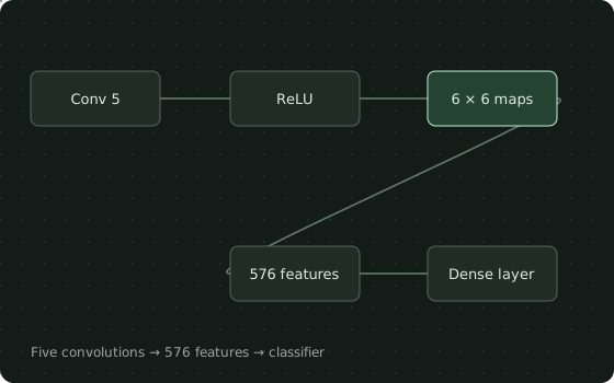
Five convolutions lead to a 16×6×6 representation and three fully connected layers. ReLU, overlapping pooling, LRN, grouped computation and dropout preserve the main architecture choices in a smaller model.
These are thumbnails of at most 8×8 cells, average-pooled from a recorded feature channel of a synthetic stripe image. The first two paths apply cross-channel LRN before pooling; the fifth pools directly. The displayed maps are untrained features and do not demonstrate ImageNet accuracy.
Min 0 · Max 0.006857
Recorded cell values
| Row / col | 0 | 1 | 2 | 3 | 4 | 5 | 6 | 7 |
|---|---|---|---|---|---|---|---|---|
| 0 | 0.006857 | 0.006857 | 0.004285 | 0 | 0 | 0.004285 | 0.006857 | 0.006857 |
| 1 | 0.006857 | 0.006857 | 0.004285 | 0 | 0 | 0.004285 | 0.006857 | 0.006857 |
| 2 | 0.006857 | 0.006857 | 0.004285 | 0 | 0 | 0.004285 | 0.006857 | 0.006857 |
| 3 | 0.006857 | 0.006857 | 0.004285 | 0 | 0 | 0.004285 | 0.006857 | 0.006857 |
| 4 | 0.006857 | 0.006857 | 0.004285 | 0 | 0 | 0.004285 | 0.006857 | 0.006857 |
| 5 | 0.006857 | 0.006857 | 0.004285 | 0 | 0 | 0.004285 | 0.006857 | 0.006857 |
| 6 | 0.006857 | 0.006857 | 0.004285 | 0 | 0 | 0.004285 | 0.006857 | 0.006857 |
| 7 | 0.006857 | 0.006857 | 0.004285 | 0 | 0 | 0.004285 | 0.006857 | 0.006857 |
Min 0 · Max 0.004077
Recorded cell values
| Row / col | 0 | 1 | 2 | 3 | 4 | 5 | 6 | 7 |
|---|---|---|---|---|---|---|---|---|
| 0 | 0.004077 | 0.004077 | 0.002446 | 0 | 0 | 0.002446 | 0.004077 | 0.004077 |
| 1 | 0.004077 | 0.004077 | 0.002446 | 0 | 0 | 0.002446 | 0.004077 | 0.004077 |
| 2 | 0.004077 | 0.004077 | 0.002446 | 0 | 0 | 0.002446 | 0.004077 | 0.004077 |
| 3 | 0.004077 | 0.004077 | 0.002446 | 0 | 0 | 0.002446 | 0.004077 | 0.004077 |
| 4 | 0.004077 | 0.004077 | 0.002446 | 0 | 0 | 0.002446 | 0.004077 | 0.004077 |
| 5 | 0.004077 | 0.004077 | 0.002446 | 0 | 0 | 0.002446 | 0.004077 | 0.004077 |
| 6 | 0.004077 | 0.004077 | 0.002446 | 0 | 0 | 0.002446 | 0.004077 | 0.004077 |
| 7 | 0.004077 | 0.004077 | 0.002446 | 0 | 0 | 0.002446 | 0.004077 | 0.004077 |
Each heatmap uses its own scale. Mint is positive, rust is negative, and the lightest color is zero. Table values are rounded to four significant digits.
Bars share one scale within this example. Values are rounded to four significant digits.
- Spatial width before pool
- 55
- Spatial width after pool
- 27
- Values after pool · all channels
- 5832
Verified by the local recipe
- The 227-pixel convention produces 55-pixel first-convolution maps and ten output logits
- LRN matches the original cross-channel sum formula, accounting for PyTorch's alpha convention
- Overlapping 3×3 stride-2 pooling matches an independent sliding-window maximum
- Grouped convolution isolates its channel groups; dropout scales survivors in training and is identity in evaluation
Download the source and run.py to reproduce these checks. Choosing an example here replays recorded values.
THE SAME MODEL, ON YOUR MACHINE
Pick up where
the graph leaves off.
Inspect an AlexNet reference with reduced widths, including grouped convolutions, local response normalization, overlapping pooling and dropout.
Use in VS Code ↗1. Save these files in one folder
2. Reproduce the example
Use Python 3.13 in a dedicated environment, matching the tested recipe. These commands are for macOS / Linux shells.
python3.13 -m venv .venv
source .venv/bin/activate
python -m pip install -r requirements.txt
python run.py
Expected output: [1,10]
Input 1: [1,3,227,227] · float32 randn · CPU / eval · seed 0
3. Open the source in TensorViz
Install the preview, open this folder in local VS Code, and choose Open as Graph above ReducedAlexNet in model.py. Select your Python environment. Save before choosing Validate.
Installation and supported setup ↗
The recipe was run with Python 3.13.13 and Torch 2.7.1. This is an untrained example; a successful shape check does not measure accuracy.
ABOUT THIS EXAMPLE
Inspect an AlexNet reference with reduced widths, including grouped convolutions, local response normalization, overlapping pooling and dropout.
Architecture · 2012
AlexNet
Five convolutions and three fully connected layers with widths 8/16/24/24/16 and 64/64/10. Uses a 227-pixel input convention, grouped conv2/4/5, LRN after the first two ReLUs, 3×3 stride-2 pools and 50% dropout.
Source, capture & limitations +
Untrained reduced-width reference. It does not recreate the original two-GPU execution, ImageNet training, augmentation or accuracy. The 227-pixel input follows the common implementation convention that yields a 55-pixel first map. CPU capture runs in evaluation mode, so dropout is inactive.
Original TensorViz teaching example. PyTorch provides the underlying operators.
No separate redistribution license has been declared for these project examples.
- Content revision
fa1d0156d71ecbf0- Source SHA-256
8e1a9aaec3de8fc9305b61411c0209c32aacbc6812aa2647307e55a6e4e05f38- Captured
- 2026-09-17 · Python 3.13.13 / Torch 2.7.1
Reduced AlexNet CPU forward, independent LRN/pooling calculations, grouped-convolution isolation and dropout-mode checks. No trained ImageNet evaluation.
Read the model manifest ↗