MODEL EXPLORER / GENERATIVE MODELS
Learn to reverse a noise schedule
How does a model learn to reverse corruption?
RECORDED NUMERICAL EXAMPLE
Corrupt once; denoise repeatedly.
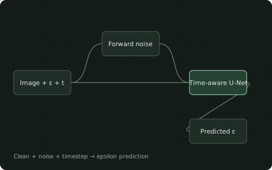
Recorded forward marginals and a separate 12-step reverse chain. The denoiser is untrained; the panel teaches DDPM scheduling, epsilon prediction and posterior sampling.
The same clean pattern and same Gaussian noise are used at each displayed t to isolate the signal/noise coefficients. These are coupled marginal examples, not consecutive forward-chain samples. The untrained prediction is compared with the actual added noise; oracle reconstruction uses known noise unavailable during generation.
Min -1 · Max 1
Recorded cell values
| Row / col | 0 | 1 | 2 | 3 | 4 | 5 | 6 | 7 |
|---|---|---|---|---|---|---|---|---|
| 0 | 0 | 0 | 0 | 0 | 0 | 0 | 0 | 0 |
| 1 | 0 | 0 | 0 | 0 | 0 | 0 | 0 | 0 |
| 2 | 0 | 0 | 1 | 1 | 1 | 1 | 0 | 0 |
| 3 | 0 | 0 | 1 | -1 | -1 | 1 | 0 | 0 |
| 4 | 0 | 0 | 1 | -1 | -1 | 1 | 0 | 0 |
| 5 | 0 | 0 | 1 | 1 | 1 | 1 | 0 | 0 |
| 6 | 0 | 0 | 0 | 0 | 0 | 0 | 0 | 0 |
| 7 | 0 | 0 | 0 | 0 | 0 | 0 | 0 | 0 |
Min -1.139 · Max 1.187
Recorded cell values
| Row / col | 0 | 1 | 2 | 3 | 4 | 5 | 6 | 7 |
|---|---|---|---|---|---|---|---|---|
| 0 | -0.0569 | 0.1814 | 0.01286 | 0.05188 | -0.2223 | -0.2517 | 0.04797 | 0.2762 |
| 1 | 0.2296 | 0.2511 | 0.1088 | -0.01921 | -0.02863 | 0.05751 | -0.1313 | -0.3035 |
| 2 | -0.06114 | 0.07756 | 1.147 | 0.9956 | 0.9916 | 0.9183 | -0.1116 | -0.04648 |
| 3 | 0.0888 | 0.0502 | 0.9959 | -1.027 | -1.139 | 1.034 | 0.2936 | 0.1104 |
| 4 | -0.01328 | 0.3288 | 0.8274 | -0.9039 | -0.9831 | 1.187 | 0.2472 | 0.1674 |
| 5 | -0.1997 | 0.1156 | 0.6953 | 1.014 | 0.9098 | 1.004 | -0.05286 | 0.005211 |
| 6 | 0.1392 | 0.06981 | -0.1281 | 0.05587 | -0.1415 | 0.2414 | -0.1888 | 0.2387 |
| 7 | -0.1274 | -0.2035 | 0.1608 | 0.1275 | 0.08359 | -0.1494 | -0.2576 | -0.2865 |
Min -1.132 · Max 1.209
Recorded cell values
| Row / col | 0 | 1 | 2 | 3 | 4 | 5 | 6 | 7 |
|---|---|---|---|---|---|---|---|---|
| 0 | -0.04773 | 0.19 | 0.02154 | 0.06549 | -0.2171 | -0.2446 | 0.05828 | 0.2833 |
| 1 | 0.2448 | 0.2652 | 0.1273 | -0.008625 | -0.02174 | 0.0712 | -0.1181 | -0.3012 |
| 2 | -0.04934 | 0.08811 | 1.174 | 1.01 | 1.008 | 0.9434 | -0.09482 | -0.04234 |
| 3 | 0.09976 | 0.05571 | 1.013 | -1.029 | -1.132 | 1.064 | 0.3056 | 0.1181 |
| 4 | 0.0008388 | 0.3467 | 0.8559 | -0.8987 | -0.9716 | 1.209 | 0.2586 | 0.1774 |
| 5 | -0.1909 | 0.128 | 0.7106 | 1.032 | 0.9271 | 1.023 | -0.04418 | 0.01844 |
| 6 | 0.1543 | 0.0804 | -0.1167 | 0.06529 | -0.1237 | 0.2584 | -0.1737 | 0.2498 |
| 7 | -0.1167 | -0.1911 | 0.176 | 0.1426 | 0.09785 | -0.1377 | -0.2505 | -0.2792 |
Each heatmap uses its own scale. Mint is positive, rust is negative, and the lightest color is zero. Table values are rounded to four significant digits.
Bars share one scale within this example. Values are rounded to four significant digits.
- Noise prediction MSE
- 1.241
- Oracle x₀ maximum error
- 2.22e-16
Verified by the local recipe
- Cumulative signal decreases; known noise reconstructs the clean image at early, middle and late steps
- Epsilon-parameterized reverse means match the analytic forward posterior
- The last reverse step adds no stochastic noise and recovers x0 with oracle epsilon
- Time conditioning affects predictions and receives gradients; one fixed-batch SGD step lowers epsilon MSE
Download the source and run.py to reproduce these checks. Choosing an example here replays recorded values.
THE SAME MODEL, ON YOUR MACHINE
Pick up where
the graph leaves off.
Inspect signal and noise coefficients, predict the added noise, and replay a complete short reverse chain with the same denoiser.
Use in VS Code ↗1. Save these files in one folder
2. Reproduce the example
Use Python 3.13 in a dedicated environment, matching the tested recipe. These commands are for macOS / Linux shells.
python3.13 -m venv .venv
source .venv/bin/activate
python -m pip install -r requirements.txt
python run.py
Expected output: [1,1,8,8]
Input 1: [1,1,8,8] · float32 randn
Input 2: [1,1,8,8] · float32 randn
Input 3: [1] · int64 ones · CPU / eval · seed 0
3. Open the source in TensorViz
Install the preview, open this folder in local VS Code, and choose Open as Graph above TinyDDPM in model.py. Select your Python environment. Save before choosing Validate.
Installation and supported setup ↗
The recipe was run with Python 3.13.13 and Torch 2.7.1. This is an untrained example; a successful shape check does not measure accuracy.
ABOUT THIS EXAMPLE
Inspect signal and noise coefficients, predict the added noise, and replay a complete short reverse chain with the same denoiser.
Training method · 2020
Denoising diffusion probabilistic models
A 12-step teaching schedule with beta from 0.02 to 0.18. Width-eight, two-resolution U-Net with a learned timestep embedding predicts epsilon for an 8 × 8 grayscale input. Reverse sampling uses fixed posterior variance.
Source, capture & limitations +
Untrained denoiser and shortened schedule, not the original image model or 1,000-step beta schedule. The terminal forward marginal is not fully Gaussian. Reverse samples illustrate arithmetic and do not establish image quality. No likelihood evaluation or learned variance; the graph shows one training forward, while the source and panel expose the repeated sampling loop.
Original TensorViz teaching example. PyTorch provides the underlying operators.
No separate redistribution license has been declared for these project examples.
- Content revision
e55f8ee8d75bece4- Source SHA-256
41018be9b51142b30ad5eb268182537f953328bcdf478c8859e71ee34b69372f- Captured
- 2026-09-17 · Python 3.13.13 / Torch 2.7.1
12-step DDPM schedule; tiny time-conditioned U-Net, oracle reconstruction, posterior-mean equivalence, final-step noise and epsilon-MSE gradient checks.
Read the model manifest ↗